|
Evaluation
of a function at the value of another (or the same) function is
called the composition of functions, denoted as (ƒ
o
g) (x) = f
(g (x)). |
| Thus,
the composition is the operation that forms a single function
from two given functions by plugging the second function into
the first for any argument. |
| The composition
of functions is only defined if the range of the first is
contained in the domain of the second function. |
|
| Examples: Given
f
(x)
= -
x2 +
4x - 1
and g (x)
= -
x
+ 1
find; |
|
a) f
(g (x)),
b) g (f
(x)),
c) g (g
(x))
and d) f
(g (-1)). |
|
| Solutions:
a) f
(g (x))
= f
(-
x
+ 1)
= -
(-x
+ 1)2 +
4(-
x
+ 1)
- 1
= - x2
-
2x + 2 |
|
b) g (f
(x))
= g (-
x2 +
4x - 1)
= -
(-x2 +
4x - 1)
+ 1
= x2 -
4x + 2 |
|
c) g (g(
x))
= g (-
x
+ 1)
= -
(-
x
+ 1)
+ 1
= x |
|
d) f
(g (-1))
= f
( -
(-1)
+ 1)
= f
(2)
= -22
+ 4 · 2 - 1
= 3 |
|
| Inverse
function
|
| The inverse function, usually written
f -1, is the function whose
domain and the range are respectively the range and domain of a given function
f, that is |
| f
-1(x)
= y if and only if
f
(y)
= x . |
| Thus, the
composition of the inverse function and the given function returns
x, which is called the
identity function, i.e., |
| f
-1(
f (x))
= x and
f (f
-1(x))
= x. |
| The inverse of a function undoes the procedure
(or function) of the given function. |
| A pair of inverse functions is in
inverse relation. |
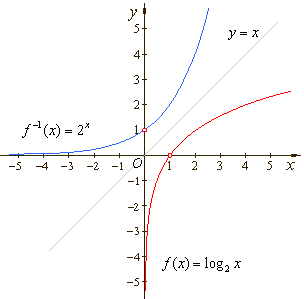
| Example: If
given
f
(x)
= log2 x
then f -1(x)
= 2x
since, |
 |
|
| Therefore,
to obtain the inverse of a function y = f
(x),
exchange the variables x
and y,
i.e., write x = f
(y)
and solve for y.
Or form the composition f
(f
-1(x))
= x and solve
for f -1. |
|
| Example: Given
y = f
(x)
= log2 x form
f -1(x). |
| Solution:
a) Rewrite
y = f
(x)
= log2 x
to x =
log2 y
and solve for y,
which gives y =
f -1(x)
= 2x. |
|
b) Form f
(f
-1(x))
= x that
is, log2
(f -1(x))
= x and
solve for f -1, which
gives f -1(x)
= 2x. |
|
| The
graphs of a pair of inverse functions are symmetrical with
respect to the line
y
= x. |
 |
|
| The
graph of a function |
| The
graph of a function ƒ
is drawing on the Cartesian plane, plotted with respect to
coordinate axes, showing functional relationship between given
variables containing all those points (x,
f (x))
which satisfy the given relation. |
| The points lying on the curve
satisfy the relation that forms the shape of the graph. |
| The
graphic representation of a function provides insight into the behavior of the
function. |
|
| Functions
behavior, properties
and characteristic points of the graph |
| To
sketch the graph of a function we should know
its properties and find out its characteristic points, as |
|
- domain and range |
|
- x-intercepts or zeros (roots) and
the y-intercept |
|
- intervals of
increasing and decreasing |
|
- continuity and discontinuity |
|
- vertical, horizontal and oblique or slant asymptotes |
|
- turning points (extremes, local or relative maximums
or minimums)
|
|
-
inflection points and intervals of concavity |
|
- symmetry (odd and even
functions) with respect to the x-axis,
y-axis, and the origin |
|
|
Domain and range |
|
The domain is
the set of values of the independent variable of a given function,
i.e., the set of all first members of the ordered pairs (x,
f (x))
that
constitute the function. |
|
The range is
the set of values that given function takes as its argument varies
through its domain. It is the image of the domain. |
|
The codomain
is the set within which the values of a function lie, as opposed to
the range, which is the set of values that the function actually
takes. |
|
Therefore, the range must be a subset of,
but may or may not be identical with the codomain. |
|
We will only consider real-valued
functions of a real variable. |
|
|
Roots or zero function
values, x-intercepts, y-intercepts |
| A
zero of a function is a value of the argument of a function at
which the value of the function is zero. |
| An
intercept
is the point at which a given function intersects with specified
coordinate axis, or the value of that coordinate at that point. |
| An
x-intercept
is the point (x,
0)
where the graph of the function touches or crosses the x-axis. |
| That
is, at the x-intercept,
the coordinate y
= 0. |
| A
zero of a function is the x
value of the x-intercept.
The
zeros (roots) of a function correspond to the x-intercepts
of the graph. |
| The
y-intercept
is the value of y
where the graph crosses the y-axis. |
| The
y-intercept
correspond to the point (0,
y) on
the y-axis
therefore,
at the
y-intercept
the coordinate x
= 0. |
|
|
Increasing/decreasing
intervals |
| A
function ƒ
is increasing on an interval if |
|
f (x1)
< f
(x2)
for each x1
< x2
in
the interval. |
| A
function ƒ
is decreasing on an interval if |
|
f (x1)
>
f (x2)
for each x1
< x2
in
the interval. |
| By looking at the graph of a function being traced out as the value of the input
variable x
increases from left to right then, if at the same time the output value
y
= f
(x) also increases, we say the function is increasing. |
| If the output value decreases as
x
increases, then we say the function ƒ
is
decreasing. |
|
| Thus,
if the slope or gradient m
of the secant line passing through the points (x1,
f (x1))
and (x2,
f (x2))
of the graph of a function
is
positive, the function is increasing (going up), as shows the
figure below. |
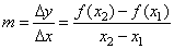 |
| where,
x2
-
x1>
0 |
| |
|
|
 |
|
| Since
the difference x2
-
x1 is
always positive, when the function is decreasing (going down), the slope will be negative. |
|
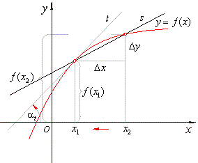
| The
instantaneous
rate of change or the derivative |
| The
ratio of the rise and the run, called the difference quotient,
that equals the value of the tangent of the angle between the
direction of the secant line and x-axis,
becomes the slope (gradient) of the tangent line as the difference Dx
tends to zero, and is called the instantaneous
rate of change or the derivative
at the point of the function. |
| For
a given function ƒ and point
(x1,
ƒ(x1)), the
derivative of ƒ at
x
= x1
is the slope of the tangent line through the point (x1,
ƒ(x1)),
i.e., f
'(x1)
= tan
at
. |
| The
gradient of a curve at a point on its graph, expressed as
the slope of the tangent line at that point, represents the rate of
change of the value of the function and is called derivative of
the function at the point, written |
| y'
=
dy/dx
=
f
'(x) |
|
| Continuity and discontinuity |
| A
function that has no sudden changes in value as the variable
increases or decreases smoothly is called continuous function. |
| Or
more formally, a real function y
=
f (x)
is continuous at a point a
if the limit of f
(x)
as x
approaches a
is
f (a). |
| If
a function does not satisfy this condition at a point it is said
to be discontinuous, or to have a discontinuity
at that point. |
|
| Vertical,
horizontal and oblique or slant asymptotes |
| A
line whose distance from a curve decreases to zero as the
distance from the origin increases without the limit is called
the asymptote. |
| The
definition actually requires that an asymptote be the tangent to
the curve at infinity. Thus, the asymptote is a line that the
curve approaches but does not cross. |
|
| Vertical
asymptote |
| The
line x =
a is a vertical asymptote
of a function f
if f
(x)
approaches infinity (or negative infinity)
as x
approaches
a
from the left or right. |
|
| Horizontal
asymptote |
| The
line y =
c is a horizontal
asymptote of a function f
if f
(x)
approaches c
as
x
approaches
infinity (or negative infinity). |
|
| Oblique or slant
asymptote |
| The
line y =
mx
+ c is a
slant or oblique asymptote of
a function f
if f (x)
approaches
the line as
x approaches infinity
(or negative infinity). |
|
-
- - -
- - - |
| The
functions that most likely have asymptotes are rational
functions. |
| So,
vertical asymptotes occur when the denominator of the simplified
rational function is equal to 0. Note that the simplified
rational function has cancelled all factors common to both the
numerator and denominator. |
|
| The
existence of the horizontal asymptote is related to the degrees
of both polynomials in the numerator and the denominator of
the given rational
function. |
| Horizontal
asymptotes occur when either, the degree of the numerator is
less then or equal to the degree of the denominator. |
In
the case when the
degree (n) of the numerator is less then the degree
(m) of the
denominator,
the x-axis
y =
0
is the asymptote. |
| If
the degrees of both polynomials, in the numerator and the denominator, are equal then,
y = an
/ bm
is the horizontal asymptote,
written as the ratio of their highest degree term coefficients respectively. |
| When
the degree of the numerator of a rational function is greater
than the degree of the denominator, the function has no
horizontal asymptote. |
|
| A
rational function will
have a slant (oblique) asymptote
if the
degree (n)
of the numerator is exactly one more than the degree (m)
of
the denominator that is if n
= m + 1. |
| Dividing
the two polynomials
that form a rational function,
of which the
degree
of the numerator
pn (x)
is exactly one more than the degree
of
the denominator qm
(x), then |
| pn
(x)
= Q (x) · qm (x) + R
=>
pn (x)
/ qm (x)
= Q (x) + R / qm (x) |
| where,
Q (x)
=
ax + b
is the quotient and R
/ qm (x)
is the remainder with constant R. |
| The
quotient Q
(x)
=
ax + b
represents the equation of the slant asymptote. |
| As
x
approaches
infinity (or negative infinity),
the remainder R /
qm (x)
vanishes (tends to zero). |
| Thus,
to find the equation of the slant asymptote, perform the long
division and discard the remainder. |
|
| The
graph of a rational function will never cross its vertical
asymptote, but may cross its
horizontal or slant asymptote. |
|
-
- - -
- - - |
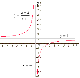
| Example: Given
the rational function |
 |
sketch
its graph. |
|
| Solution:
The
vertical asymptote can be found by finding the root of the
denominator, |
|
x + 1 = 0 =>
x = -1
is the vertical asymptote.
|
|
The
horizontal asymptote is the ratio of their
highest degree term coefficients since
the degree of polynomials in the numerator and denominator are equal,
|
| |
 |
is the
horizontal asymptote. |
|
|
The graph of the given rational function is translated equilateral (or rectangular)
hyperbola shown below.
|
| The
rational function of the
form
|
 |
can
be rewritten into
|
|
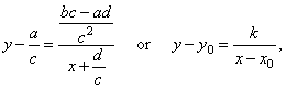 |
|
|
| where, x0
and y0
are asymptotes and k
is constant. |
|
 |
|
|
Therefore, values of the vertical and
the horizontal asymptote correspond to the coordinates of the horizontal and the vertical translation
of the source equilateral hyperbola y
= k/x, respectively.
|
|
|
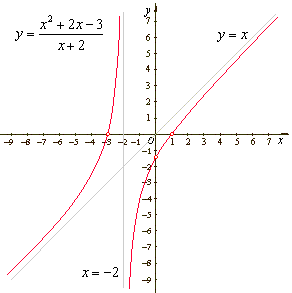
| Example: Given
the rational function |
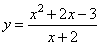 |
sketch
its graph. |
|
| Solution:
The
vertical asymptote can be found by finding the root of the
denominator, |
|
x + 2 = 0 =>
x = -2
is the vertical asymptote.
|
| Since
the
degree
of the numerator is exactly one more than the degree of
the denominator the given rational function has the slant
asymptote. |
| By dividing the
numerator by the denominator |
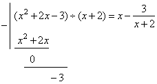 |
| obtained is
the slant asymptote y
= x |
| and
the
remainder
3/(x + 2) that vanishes as x
approaches
positive or negative infinity. |
|
 |
|
|
|
| Stationary
points and/or critical points |
| The
gradient of a curve at a point on its graph, expressed as
the slope of the tangent line at that point, represents the rate of
change of the value of the function and is called derivative of
the function at the point, written dy/dx
or f
'(x). |
| At
points of the graph where function changes from increase to
decrease, the slope
of the tangent line changes from
positive to negative values respectively, passing through zero value. |
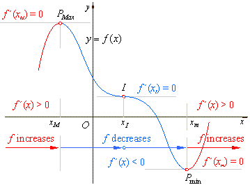 |
| The
points of the graph of a function at which the tangent lines are
parallel to the x-axis,
and therefore the derivative at these points is zero, are called
the stationary
points. |
| There
are three different types of stationary points: maximum points,
minimum points and points of horizontal inflection. On the above graph
the stationary points are
denoted as,
PMax, I
and Pmin. |
| The
graph reaches a local (or relative)
maximum
when gradient changes from positive through
zero to negative. |
| The
graph reaches a local (or relative)
minimum when gradient changes from
negative through
zero to positive. |
| A
local maximum
is a value of the function greater than any adjacent value,
i.e., in its immediate area it is the
highest point,
but it may not be the greatest value of the function over its
whole range. |
|
| The
endpoints of intervals of monotonicity are places where
function stops increasing and starts decreasing or vice versa. |
| A
function f
(x)
can change from increasing to decreasing (or vice
versa) at values where f
'(x)
= 0 or f
'(x)
is undefined. |
| Note that these are only potential places where the graph can change from increasing to decreasing (or vice versa) since it is possible that the function may not change at those values, as for example at the point
xI (where
f
'(x)
= 0), in the above figure or, as in case of the rational
functions from the above two examples, at the vertical asymptotes (where
f
'(x)
is undefined). |
| If
f (x)
is
defined at x
= c and either f
'(c)
= 0
or
f
'(c)
is not defined, then x
= c
is called a critical
value of the function f
(x),
and its point (c,
ƒ(c))
is called a critical point. |
| Therefore,
a critical point may be a local maximum, a
local minimum, or neither. |
| The
critical point is neither a maximum nor a minimum if the
function does not change from increasing to decreasing (or vice
versa) at the critical point, as at the point xI
in the above figure. |
| For
a given function ƒ and point
(c,
ƒ(c)), the
derivative of ƒ at
x
= c is the slope of the tangent line through the point
(c,
ƒ(c)),
i.e., f
'(c)
= tan
at
. |
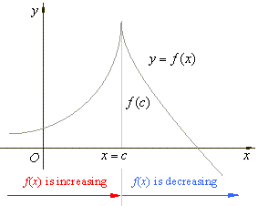
|
| The
function value f
(c)
in
the right figure is defined and the derivative
at x
= c
is undefined, therefore the point (c,
f (c))
is a critical point. |
|
| As
f
(x)
is increasing before x
= c
and decreasing after x
= c,
the point (c,
f (c))
is a local maximum. |
|
 |
|
|
| Turning points (extremes, local or relative maximums
or minimums)
|
| A
stationary
point at which the gradient (or the derivative) of a function
changes sign, so that its graph does not cross a tangent line
parallel to x-axis,
is called the tuning
point. |
| Thus,
a turning point is
a critical point where the function turns from being increasing
to being decreasing (or vice versa),
i.e., where its derivative
changes
sign. |
 |
| A
local (or relative) maximum
is a point where the function turns from being increasing to
being decreasing, i.e., where its derivative changes sign from
positive to negative. |
| Notice
that, as we travel through
the maximum turning point from left to right, the
derivative (the slope of the tangent to the curve) is
decreasing, i.e.,
f
'(x) changes
from positive through zero to negative as x
increases. |
| Thus,
if the derivative of a function is decreasing over an interval,
the graph of the function is concave down. |
| A
local (or relative) minimum
is a point where the function turns from being decreasing to
being increasing, i.e., where its derivative changes sign from
negative to positive. |
| Thus,
as we travel through the minimum turning point from left to
right, the derivative
is increasing, i.e.,
f
'(x) changes
from negative through zero to positive as x
increases. |
| Therefore,
if the derivative of a function is increasing over an interval,
the graph of the function is concave up. |
|
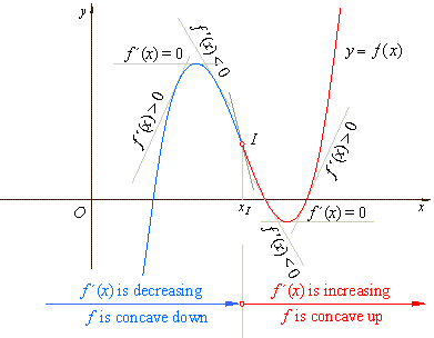
| Inflection points and intervals of concavity |
| A
point on a curve at which it crosses its tangent, and concavity
changes from up to down or vice versa, is called the point of
inflection, as shows the above figure. |
| The
graph is concave up on an open interval where the slope
increases and concave down on an open interval where the slope
decreases. |
| Therefore,
the
points on a curve that join arcs of opposite concavity are
points of inflection. |
| If
the gradient of the function does not change sign at the
stationary point, then it is a point of horizontal inflection. |
|
| Symmetry
of a function, parity - odd and even functions
|
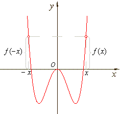
| A
function f
that changes neither sign nor absolute value when the sign of
the independent variable is changed is even,
so that,
f (x)
= f (-x). |
| Therefore,
the
graph of such a function is symmetrical with respect to the y-axis,
as is the graph shown in the left figure below. |
 |
 |
| The
graph of an even function. |
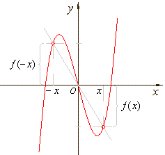
The
graph of an odd function. |
|
| A
function f
that changes sign but not absolute value when the sign of the
independent variable is changed is odd,
so that,
f (x)
= -
f (-x).
That is,
for each x
in the
domain of f,
f (-x)
= -
f (x).
|
| Therefore,
the
graph of such a function is symmetrical with respect to the
origin, as is the graph shown in the right figure above. |
|
| Transformations
of original or source function |
| How
some changes of a function notation affect the
graph of the function |
| Some
changes
in a function expression
(or an equation/formula)
do not affect the shape or the form of the
graph of the original
or the given function y
= f (x). |
| Such
changes include use of geometrical transformations to the graph
of the function, like
translations (or shifts) of the graph of the
original function in
the direction of the coordinate axes, or its reflection across
the axes. |
|
| Translations
of the graph of a function
|
| The
graph of a translated function y
= f (x - x0)
is
obtained |
| translating (shifting) the graph of its
original or source function y
= f (x)
horizontally by
x0
units to the right. |
| The
graph of a translated function y
= f (x) +
y0
or y
- y0
= f (x) |
|
is obtained translating (shifting) the graph of its
original function y
= f (x)
vertically by
y0
units up. |
| The
graph of a translated function |
| y
= f (x - x0)
+ y0 or
y
- y0
= f (x - x0)
|
| is
obtained translating (shifting) the graph of its
original function y
= f (x)
in both directions of the coordinate axes, horizontally by
x0
units
to the right and vertically
by
y0
units up. |
|
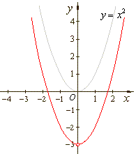
| Example: Draw
the graphs of the given three quadratic polynomials, |
| a)
y
= x2 + 4x + 4 = (x + 2)2,
b)
y
= x2 -
3
and
c)
y
= x2 + 4x + 1
or
y
+ 3 = (x + 2)2 |
| as
the translations of the same source quadratic y
= x2. |
 |
 |
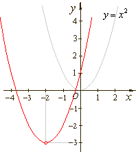 |
| a)
y
= (x + 2)2 |
b)
y
= x2 -
3 |
c)
y
+ 3 = (x + 2)2 |
|
|
| Reflections
of the graph
of a function - changing polarity of variables |
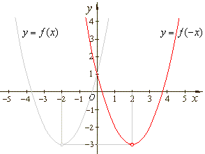
|
Change of the sign of
the independent variable of a function, denoted as y
= f (-x),
reflects the graph of the given (original) function
y
= f (x)
across the y-axis. |
| Change
of the sign of the function, denoted
as y
= - f
(x),
reflects the graph of the given function y
= f (x)
across the x-axis. |
| Changes
of the signs of both, independent variable and the function, denoted as
y
= - f
(-x),
reflect
the graph of the given function y
= f (x), across the y-axis
and the x-axis. |
|
| Example: Given quadratic
polynomial y
= f (x) = x2 + 4x + 1
or
y
+ 3 = (x + 2)2,
transform to: |
|
a) y
= f (-x),
b)
y
= - f
(x)
and c) y
= -
f (-x),
and draw corresponding graphs. |
|
| Solution:
a)
y
= ƒ(-x)
= (-x)2 + 4(-x) + 1
= x2 - 4x + 1
or
y + 3 = (x
-
2)2 |
|
b) y
= -ƒ(x)
= -(x2 + 4x + 1)
= -x2
-
4x - 1
or
y -
3 = -(x + 2)2 |
|
c) y
= -ƒ(-x)
= -((-x)2 + 4(-x) + 1)
= -x2 +
4x - 1
or
y - 3 =
-(x
-
2)2 |
 |
 |
| a)
y
+ 3 = (x - 2)2 |
b)
y
- 3 =
- (x + 2)2 |
|
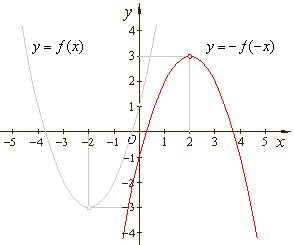 |
| c)
y
= -x2 + 4x
- 1
or
y
- 3 =
- (x
- 2)2 |
|
|
|
|
|
|
|